If a quiet musical passage is 50 dB at your listening chair and a loud passage reaches 90 dB, that is a 40 dB difference in level. Or 40 dB of dynamic range.

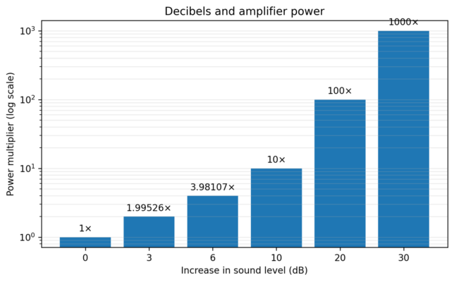
But remember: the decibel scale is logarithmic. For amplifier power, an increase of 3 dB requires about twice the power, assuming everything else stays equal.

10 dB requires ten times the power.

20 dB requires 100 times the power.

And 30 dB requires 1,000 times the power.

That is the first fact to keep in mind. Relatively modest-looking changes in dB can create enormous changes in amplifier power demand.

How Dynamic Is Live Music?

Before talking about recordings, think about live music. And immediately we have to ask: live music of what kind?

A classical guitar is not a symphony orchestra.

A string quartet is not a drum kit.

A jazz trio in a small club is not an amplified rock concert.

So, there is no single dynamic-range number for live music.

Acoustic music can move from sounds that are only modestly above the ambient noise of the concert hall to very high short-term peaks. A full orchestra can change dramatically between pianissimo and fortissimo. Individual events such as bass-drum strikes, hard piano attacks, and close brass can produce much larger instantaneous peaks than the long-term average level of the performance.

We use classical music as an example because it can be very dynamic despite lack of amplification. But the principles apply to any music.

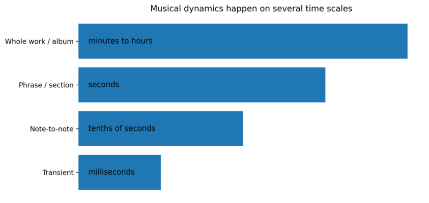
That distinction between average and instantaneous level is the key to this entire discussion. Now, music has dynamic structure on several time scales. There is the difference between a quiet movement or section of the music and a loud movement or phrase or section. There is the difference between a verse and a chorus, or a soft phrase and a loud phrase. There is the difference from note to note. And there is the very brief transient at the beginning of a drum strike, piano note, or plucked string.

All of these are dynamics.

But they do not all ask the same question about your stereo system.

There Is No Single Dynamic Range (DR) Number

Suppose I tell you that a recording has 20 dB of dynamic range. What exactly do I mean?

Do I mean the quietest meaningful section is 20 dB below the loudest section?

Do I mean the loudest instantaneous peak is 20 dB above the average signal level?

Or do I mean that most of the program loudness falls within a 20-unit range?

These are different measurements. Professional loudness practice recognizes this. The ITU BS.1770 standard defines program loudness and true-peak level as separate measurements. The European Broadcasting Union’s Loudness Range, or LRA, describes the statistical distribution of loudness over time. It deliberately avoids allowing one extreme outlier to define the whole program.

That makes sense when we want to describe generally and typically how much the apparent loudness of a work changes. But an amplifier cannot ignore an outlier. The single biggest peak may be the exact event that clips the amplifier.

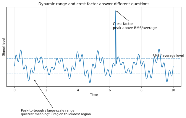
So here is the most important conceptual distinction we need to understand about the real music or the recording:

Large-scale dynamic range tells us about the contrast between quieter and louder musical material.

Crest factor tells us how high the signal peaks rise above its RMS (roughly the average) level over a defined, longer measurement interval.

For amplifier headroom, crest factor is often the more immediately useful idea.

Crest Factor: The Number Audiophiles Should Understand

The Audio Engineering Society defines crest factor as the ratio of peak level to RMS level measured over a specified time interval. In dB, we can think of it as the height of the peak above the RMS level. The AES notes that recorded music “commonly” has crest factors in roughly the 12-to-20 dB range.

But particular recordings can fall below or above that range.

And logically, audiophiles want to talk about the upper end for system planning, because some minimally compressed classical recordings and transient-rich acoustic recordings can present peak-to-average relationships in the low-to-mid 20s. These levels are outside the AES “common” DR.

This is where amplifier power becomes interesting.

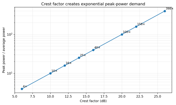
Suppose the average musical signal requires 1 watt. A peak 10 dB above the average requires ten times the power, or 10 watts. A 20 dB peak requires 100 times the power, or 100 watts. A 26 dB peak is almost 400 times the average power, or 400 watts.

One watt average can therefore be associated with an instantaneous peak demand approaching 400 watts. That does not mean the amplifier is delivering 400 watts continuously. It may be asked to do it for a tiny fraction of a second. But if the amplifier cannot supply the required voltage and current, even for a short period, the peak clips.

How Crest Factor Tends to Differ by Music Type

We should be careful about assigning fixed crest factors to musical genres.

Genre does not determine mastering. Two releases of the same album can have different dynamics. A heavily limited classical crossover recording may have less crest factor than a carefully mastered jazz recording.

Still, there are useful broad tendencies.

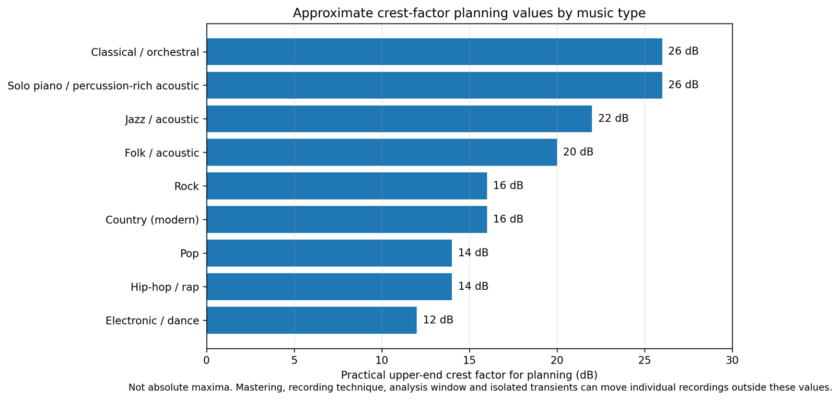
For practical system-planning examples, from measured data, we find upper-end crest factors as follows:

Very dynamic orchestral recordings: 24-26 dB

Transient-rich solo piano and percussion-heavy acoustic recordings: mid-20s

Acoustic jazz: roughly 20 to 22 dB.

Folk and other lightly processed acoustic recordings: 18 to 20.

Rock and modern country are often lower: 14-to-16 dB upper-end planning range.

Pop and hip-hop are often around 12 to 14 at the dynamic end of modern releases.

Electronic dance music is commonly lower still because high average density is often part of the production aesthetic.

These are not absolute maxima.

And here we want to make an important correction to a phrase that is sometimes used too casually. The AES does not say that 20 dB is a practical limit for music. Its Pro Audio Reference says that music has a wide crest-factor range of roughly 12 to 20 dB. That is a descriptive range for common program material. It is not a recommendation that an audiophile should design a system around a 20 dB ceiling.

Why does that matter? Because the AES cannot possibly know the listener’s budget, loudspeaker sensitivity, room, listening distance, preferred genres, specific tracks, or willingness to trade cost and size for headroom. Those are system-design choices. If the music you care about can produce 26 dB crest factors, designing only for 20 dB means accepting 6 dB less peak headroom. 6 dB is about four times the amplifier power. At the same average listening level and with the same loudspeaker, a system that needs 100 watts to cover 20 dB peaks would need about 400 watts to cover 26 dB peaks. A 24 dB peak requires about two-and-a-half times the power of a 20 dB peak. And a 30 dB peak would require ten times the power.

So there are really two legitimate design questions. One is: what amount of headroom is practical for the system I am willing to buy? The other is: what amount of headroom would be required to preserve the largest peaks in the music I actually play? Those are not the same question. The first introduces a budget and equipment constraint. The second starts with the music. For an audiophile trying to reproduce the maximum dynamics of very wide-crest-factor genres, the second question is the more honest starting point.

They are planning values.

The measurement window for DR matters. The mastering matters. And one isolated drum transient can produce a larger instantaneous crest factor than the recording as a whole.

The larger point is that the music you play changes the headroom problem.

From Crest Factor to Risk: How Often Will the Amplifier Run Out of Power?

The phrase “music commonly has 12 to 20 dB of crest factor” is useful as a broad description, but it is incomplete for amplifier sizing because “commonly” is not a probability. A consumer needs a different question: with 20, 24, 26, or 30 dB of available peak headroom, how likely is the music to exceed the system’s capability?

The ideal data would be a genre-conditioned exceedance curve: P(crest factor > x). The literature does not yet provide exactly the audiophile clipping-risk table we want. AES describes music broadly as having a wide 12–20 dB crest-factor range; AES75/M-Noise reflects analysis of a large variety of program material and recognizes frequency-dependent crest behavior; and Kirchberger and Russo analyzed 1,000 songs with percentile-based level distributions and found systematic genre differences. Those are useful anchors, but not a direct probability-of-clipping dataset.

The accompanying curves are therefore explicitly conceptual and estimated. They model three broad program families: dense modern pop/rock/electronic; acoustic/jazz/lightly processed; and classical or other transient-rich acoustic music. The curves are intended to show the likely shape and relative ordering of the risk, not to claim measured probabilities.

The important engineering implication is quantitative. Relative to a 20 dB design point, 24 dB of headroom requires 2.51 times the peak amplifier power; 26 dB requires 3.98 times; and 30 dB requires 10 times. The additional amplifier is buying a smaller probability that an unusually large musical peak will clip.

That reframes the power question. There is no single correct wattage independent of risk. The listener is choosing how far into the estimated tail of the musical peak distribution the system should remain linear.

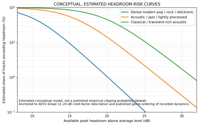
To illustrate reading this chart, look at the blue curve. If your system has a peak headroom of 15 dB (on the horizontal axis), then 10% (10 to the first power) of recordings will exceed your system DR as indicated on the vertical. Probably maybe. Remember, these are estimates.

Average Listening Level Plus Crest Factor Sets the Peak Target

Now we can build the power calculation correctly.

Start with the average level at which you listen.

Then add the crest factor of the music.

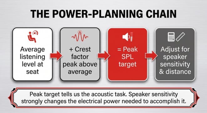
Average listening level plus crest factor equals peak SPL target.

This is the acoustic task.

Then we ask how difficult that task is for the loudspeaker and amplifier.

Speaker sensitivity matters because a more sensitive loudspeaker produces more acoustic output for a given electrical input.

Listening distance matters because sound power is reduced with greater distance.

The number of speakers playing matters.

Room reflections matter.

And the loudspeaker’s real impedance and phase angle matter to the amplifier.

But the basic reasoning chain is simple:

Average listening level + musical crest factor = peak SPL target.

Then, speaker sensitivity and the listening geometry help determine how much amplifier power is needed to reach that target.

What the Same Headroom Costs in Three Different Systems

Now let us translate headroom into watts, but this time we will make the assumptions explicit.

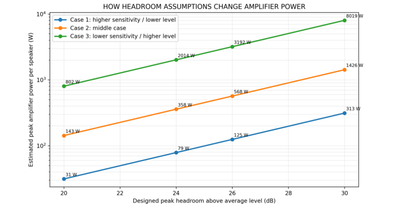
Case One uses 89 dB-sensitive speakers, a 2.5-meter listening distance, and a 79 dB average listening level.

Case Two uses 87 dB-sensitive speakers, a 3-meter listening distance, and an 82 dB average level.

Case Three uses 85 dB-sensitive speakers, a 4-meter listening distance, and an 85 dB average level.

For this simplified comparison, sensitivity is treated as one watt at one meter. We give a stereo pair a 3 dB contribution. We use inverse-distance loss of 20 log base ten of distance. We assume no extra room gain and a benign loudspeaker impedance. The figures are peak watts per speaker.

At 20 dB of headroom needed, the three systems require approximately 31 watts, 143 watts, and 802 watts per speaker. For peaks.

At 24 dB headroom, the requirements rise to about 79 watts, 358 watts, and 2,014 watts.

At 26 dB headroom, they rise to about 125 watts, 568 watts, and 3,192 watts.

At 30 dB headroom, the simplified calculation gives roughly 313 watts, 1,426 watts, and 8,019 watts.

The last numbers are intentionally startling. They do not mean that a conventional loudspeaker will necessarily survive or remain linear at those levels. In many systems, driver excursion, thermal compression, impedance, or amplifier current capability will become the limit first. In theory, however, note that Case 2, which is a typical speaker in a typical medium-sized room at a typical distance with a reasonable average level, requires 568 watts per channel to deliver a 108 dB peak.

But that is the lesson. The music-risk curve may be the same, while the watts required to move farther into its tail can differ by orders of magnitude because sensitivity, distance, and average listening level are different.

Two Systems That Look Similar — But Are Not

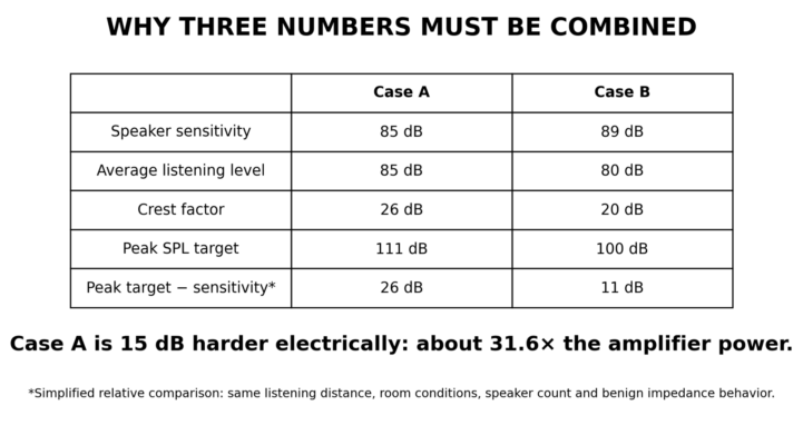
Let’s expand this with two more examples. Case A uses a speaker with 85 dB sensitivity, the listener plays music at an average level of 85 dB at the chair, and the music has a 26 dB crest factor. 85 + 26 = 111, so the system must reproduce 111 dB peaks at the chair if we want to preserve those peaks without clipping.

Now consider Case B. Here, the speaker has 89 dB sensitivity, the average listening level is 80 dB, and the recording has a 20 dB crest factor. 80 + 20 = 100, so Case B needs 100 dB peaks. Already, Case A has an 11 dB higher acoustic peak target — but Case A also uses a speaker that is 4 dB less sensitive. Under the same simplified distance and room assumptions, the electrical difficulty is therefore about 15 dB greater, and 15 dB corresponds to approximately 32 times the amplifier power. Thirty-two times.

That is the point we want to emphasize. We cannot look only at speaker sensitivity, only at average listening level, or only at a DR or crest-factor number; the required headroom is created by the combination. Case A — low sensitivity, high listening level, very high crest factor — and Case B — higher sensitivity, lower listening level, lower crest factor — are radically different amplifier problems.

The One-Watt, Hundreds-of-Watts Paradox

This explains why two audiophiles can measure their systems and reach apparently contradictory conclusions.

One says: I almost never use more than a few watts. The other says: you need a 300-watt amplifier. Both statements can be correct.

Imagine that the average musical level corresponds to two watts. With a 20 dB crest factor, the peak-to-average power ratio is 100 to one. Two watts average means 200 watts peak. With a 26 dB crest factor, the power ratio is nearly 400 to one.

Two watts average would imply a theoretical peak demand approaching 800 watts.

Again, this is a simplified electrical illustration.

Real loudspeaker impedance changes with frequency. The acoustic contribution of two speakers is not the same as one. Rooms add reflected energy. And loudspeakers may reach excursion or compression limits before the amplifier reaches the calculated wattage. Or not.

But the scale of the relationship is real. This is why amplifier headroom can matter when average power is modest. And average listening levels matter in defining what modest power level two different users employ (2 watts vs 500 mW – both might be summarized as “typically 1 watt”).

Peak-to-Trough Range and Crest Factor Create Different System Problems

Imagine two recordings.

Recording A is an orchestral work. It contains very quiet passages, moderate average levels, and occasional enormous peaks.

Recording B is heavily compressed rock. There are few genuinely quiet passages. The average level is high, and the peaks stay relatively close to the average.

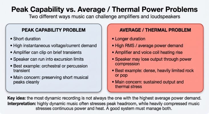
The orchestral recording may have a much larger total dynamic range and a much larger crest factor. Its challenge is peak capability. The amplifier needs voltage and current headroom for brief events. The woofer may need substantial excursion on low-frequency peaks.

The compressed rock recording creates a different problem. Its peak target may be lower, but its average power demand can be much higher. Average listening level may be much higher as well. The amplifier is asked to deliver substantial output for longer periods. The voice coil heats. Its resistance rises. Acoustic efficiency can fall. That is power compression.

So, the most dynamic recording is not necessarily the recording with the highest average power demand. One recording may be difficult because of instantaneous peaks. Another may be difficult because of sustained RMS power and heat.

Dynamic Range by Musical Genre

Across groups of commercial recordings, research has found broad genre patterns.

Modern pop, rap, and rock recordings generally show smaller measured dynamic ranges than classical genres such as opera and orchestral music. Quoted DR may be “typical,” not crest factor.

Jazz tends to fall between the modern popular and classical groups.

And this is a tendency, not a rule.

The recording and mastering process can overwhelm the genre tendency.

Compression is also not automatically bad. It is an artistic tool. It can create sustain, density, and rhythmic character. The sound of a compressed electric guitar is part of the language of rock.

The problem for our discussion is simply that compression changes the relationship between peak and average level.

When peaks are limited, and the program is raised in level, average power increases while crest factor falls. That is why two recordings can both peak near the digital ceiling and still make completely different demands on the playback system.

What Should an Audiophile Actually Know?

For system planning, we want four numbers or ideas.

First: average listening SPL at the chair.

Second: the max crest factor, or peak-above-average behavior, of the kind of music you care about reproducing.

Then combine these two: average listening level plus max crest factor gives the peak SPL target.

From there, speaker sensitivity, distance, two-speaker contribution, room conditions, and the loudspeaker’s electrical load determine how demanding that peak target is for the amplifier.

This is a much better way to think about power than asking: how many watts does this speaker need?

Conclusion

Dynamic range sounds like a simple concept. The difference between loud and soft. But for audio reproduction, we have to ask a more precise question.

Are we talking about the quietest meaningful passage compared with the loudest passage?

The distribution of program loudness over time? Or the height of the instantaneous peaks above the average signal level? For understanding musical contrast, large-scale loudness range matters. For understanding whether quiet passages disappear into room noise, total range matters. But for understanding amplifier headroom, crest factor is enormously important. And it must be combined with the level at which you actually listen and the sensitivity of your loudspeakers.

That is why one audiophile can be perfectly happy with 30 watts, and another can clip a 300-watt amplifier.

The goal of power is not simply to play loud. To borrow from an old Cerwin-Vega ad: “dynamic is beautiful if it’s clean.”

The goal is to preserve the musical relationship between average level and the peak. Between the body of a note and its attack. Between the orchestra gathering energy and the instant it finally releases. It is how freely the music can change.

Estimated-risk-model note:

The literature reviewed here does not publish the exact genre-by-genre crest-factor exceedance curves needed to calculate the probability that a home stereo amplifier will clip. The curves in this article are conceptual estimates informed by AES’s broad crest-factor description, AES75/M-Noise program analysis, and published percentile-based genre comparisons. They are intended for system-planning intuition, not as measured actuarial probabilities.

References

• ITU-R BS.1770-5 (2023). Defines algorithms for program loudness and true-peak audio level as separate descriptors.
• EBU Tech 3342 v2.0. Defines Loudness Range, or LRA, as a statistical description of program loudness variation rather than a simple quietest-sample to loudest-sample subtraction.
• AES Pro Audio Reference: Crest Factor. Defines crest factor as peak relative to RMS over a specified interval and notes that music commonly falls around 12–20 dB.
• Kirchberger and Russo (2016). A cross-genre analysis found generally smaller measured dynamic ranges in popular genres such as rock and rap than in classical genres such as opera and orchestra; jazz was broadly intermediate.